✅作者简介:热爱科研的Matlab仿真开发者,修心和技术同步精进,matlab项目合作可私信。
🍎个人主页:Matlab科研工作室
🍊个人信条:格物致知。
更多Matlab仿真内容点击👇
⛄ 内容介绍
可再生能源 (RES) 和储能系统 (ESS) 在微电网中的集成为最终用户和系统运营商带来了潜在利益。然而,RES 的间歇性问题和 ESS 的高成本需要对微电网的经济运行进行审查。本文介绍了一种用于微电网的双层预测能量管理系统 (EMS),该系统具有由电池和超级电容器组成的混合 ESS。结合充电深度和寿命方面的混合 ESS 退化成本,电池和超级电容器的长期成本被建模并转化为与实时操作相关的短期成本。为了以最低的运营成本保持较高的系统稳健性,提出了一种分层调度模型来确定有限时间范围内微电网中公用事业的调度,其中上层 EMS 最小化总运营成本,下层 EMS 消除由预测误差引起的波动。仿真研究表明,可以在两个控制层使用不同类型的能量存储来实现多个决策目标。包含不同定价方案、预测范围长度和预测准确性的场景也验证了所提出的 EMS 结构的有效性。仿真研究表明,可以在两个控制层使用不同类型的能量存储来实现多个决策目标。包含不同定价方案、预测范围长度和预测准确性的场景也验证了所提出的 EMS 结构的有效性。仿真研究表明,可以在两个控制层使用不同类型的能量存储来实现多个决策目标。包含不同定价方案、预测范围长度和预测准确性的场景也验证了所提出的 EMS 结构的有效性。
⛄ 部分代码
clear;
clc;
addpath('./datasets' , './examples', './misc', ...
'./model_func', './print_func', './process_func', './user_func' );
%% Do not modify this part
tol_opt = 1e-8;
opt_option = 1;
iprint = 5;
[tol_opt, opt_option, iprint, printClosedloopDataFunc]...
= fcnChooseAlgorithm(tol_opt, opt_option, iprint, @printClosedloopData);
%Do not modify this part END
%% Initialization
global fst_output_data ;
global snd_output_data ;
fst_output_data = [];
snd_output_data = [];
fst = fcnSetStageParam('fst');
snd = fcnSetStageParam('snd');
%import datasets
fprintf('Import data....');
importDataTic = tic;
mpcdata = fcnImportData('data/data_all.csv','data/price_seq_RT.csv');
pv_5m_data_all = xlsread('data/pv_5m_5percent.xlsx');
wind_5m_data_all = xlsread('data/wind_5m_5percent.xlsx');
importDataTic = toc(importDataTic);
fprintf('Finish. Time: %4fs\n', importDataTic);
clearvars importDataTic;
% Step (2) of the Nonlinear MPC algorithm:
options = fcnChooseOption(opt_option, tol_opt, fst.u0);
%% Start iteration: first layer
fst.mpciter = 0; % Iteration index
while( fst.mpciter < fst.iter )
% Read data
fst.load = mpcdata.load(fst.mpciter+1:fst.mpciter+fst.horizon,:);
fst.PV = mpcdata.PV(fst.mpciter+1:fst.mpciter+fst.horizon,:);
fst.wind = mpcdata.wind(fst.mpciter+1:fst.mpciter+fst.horizon,:);
fst.price = mpcdata.price(fst.mpciter+1:fst.mpciter+fst.horizon,:);
% FIRST mpc calculation
tic
[fst.f_dyn, fst.x_dyn, fst.u_dyn] = fst_mpc( fst, fst_output_data );
toc
%Second Layer Initialization
snd.pv_all = [];
snd.load_all = [];
snd.price_all = [];
snd.u0_ref = [];
if snd.flag == 0 % initial state of supercap
snd.xmeasure = [fst.x_dyn(1,:),50];
else
snd.xmeasure = [fst.x_dyn(1,:),snd.xmeasure(1,3)];
end
for i = 1:1:snd.from_fst %take care the value of MPCITER
snd.load_all = [snd.load_all ; repmat(mpcdata.load(fst.mpciter+i),snd.iter,1)];
snd.price_all = [snd.price_all;repmat(mpcdata.price(fst.mpciter+i), snd.iter,1)];
snd.u0_ref = [snd.u0_ref, repmat([ fst.u_dyn(:,i);0],1,snd.iter)]; % reference of variables in snd layer
end
snd.u0 = snd.u0_ref(:,1:snd.horizon);
%% Start iteration: second layer
snd.mpciter = 0; %iteration Index
snd.option = options;
while (snd.mpciter < snd.iter)
% data changed in every 5 min
snd.PV = pv_5m_data_all(snd.mpciter+1+12*fst.mpciter, 1:12)';
snd.wind = wind_5m_data_all(snd.mpciter+1+12*fst.mpciter, 1:12)';
% data not changed in every 5 min
snd.load = snd.load_all(snd.mpciter+1:snd.mpciter+snd.horizon,:);
snd.price = snd.price_all(snd.mpciter+1:snd.mpciter+snd.horizon,:);
%%
%SECOND mpc calculation
[snd.f_dyn, snd.x_dyn, snd.u_dyn] = snd_mpc( snd, snd_output_data );
%Next iteration:
snd.u0 = shiftHorizon(snd.u_dyn); %Estimated control variables
snd.xmeasure = snd.x_dyn(2,:);
snd.mpciter = snd.mpciter+1;
snd.x = [ snd.x; snd.x_dyn(1,:) ];
snd.u = [ snd.u; snd.u_dyn(:,1)' ];
end
snd.flag = 1; %
%Second layer ends
%FIRST: Next iteration
fst.u0 = shiftHorizon(fst.u_dyn); %Estimated control variables
fst.xmeasure = snd.xmeasure(1,1:2); % From the second layer if second layer EXISTS
% fst.xmeasure = fst.x_dyn(2,:); %Estimated state variables, if second layer does not exist
fst.mpciter = fst.mpciter+1;
%FIRST: Next iteration ends
fst.f = [fst.f, fst.f_dyn];
fst.x = [ fst.x; fst.x_dyn(1,:) ];
fst.u = [ fst.u; fst.u_dyn(:,1)' ];
end
esspower=value(fst.u);
esssoc=value(fst.x);
esspower1=value(fst.u_dyn);
esssoc1=value(fst.x_dyn);
miwind=value(fst.wind);
miPV=value(fst.PV);
miload=value(fst.load);
% costallcal=value(fst.f)
% costvalu=value(costallcal.)
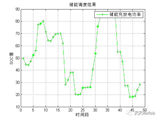
figure(1)
% yyaxis left
bar(esssoc(:,1),'linewidth',0.001)
xlabel('时间段')
ylabel('储能充放电功率')
% yyaxis right
plot(esssoc(:,2),'-g*','linewidth',1.25)
grid
xlabel('时间段')
ylabel('SOC值')
title('储能调度结果')
legend('储能充放电功率','储能SOC值')
figure(2)
plot(esspower(:,1),'-r*','linewidth',1.25)
grid
xlabel('时间段')
ylabel('generation power')
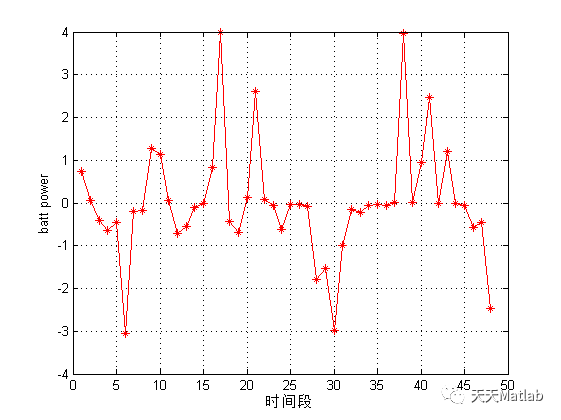
figure(3)
plot(esspower(:,2),'-r*','linewidth',1.25)
grid
xlabel('时间段')
ylabel('batt power')
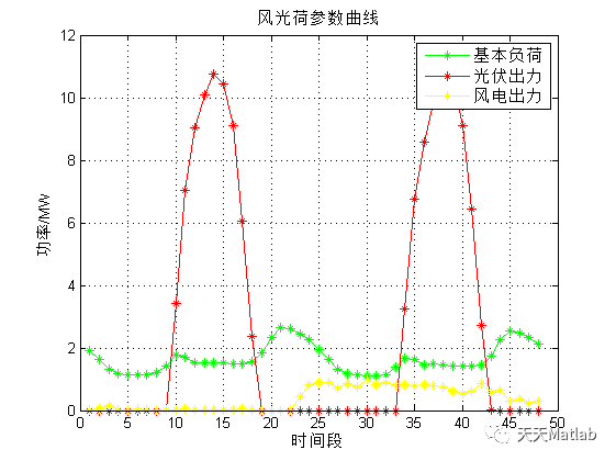
figure(4)
plot(miload,'-g*','linewidth',1.15)
hold on
grid
plot(miPV,'-r*','linewidth',1.15)
hold on
plot(miwind,'-y*','linewidth',1.15)
xlabel('时间段')
ylabel('功率/MW')
title('风光荷参数曲线')
legend('基本负荷','光伏出力','风电出力')
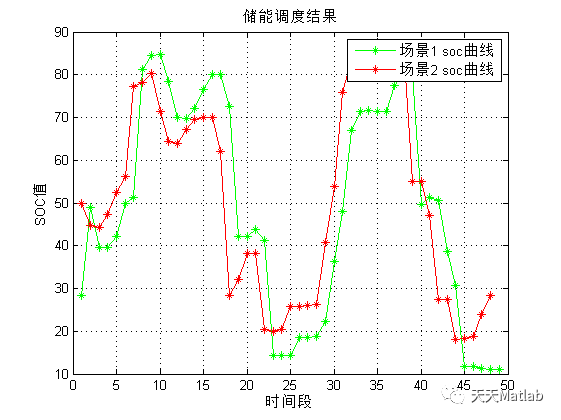
figure(5)
plot(esssoc1(:,2),'-g*','linewidth',1.25)
grid
hold on
plot(esssoc(:,2),'-r*','linewidth',1.25)
legend('场景1 soc曲线','场景2 soc曲线')
xlabel('时间段')
ylabel('SOC值')
title('储能调度结果')
figure(6)
plot(esssoc1(:,1),'-g*','linewidth',1.25)
grid
hold on
plot(esssoc(:,1),'-r*','linewidth',1.25)
legend('场景1 功率曲线','场景2 功率曲线')
xlabel('时间段')
ylabel('充放电功率')
title('储能调度结果')
%rmpath('./datasets' , './examples', './misc', ...
% './model_func', './print_func', './process_func', './user_func' );
% save('exportData/fst.mat','fst');
% save('exportData/snd.mat','snd');
% save('exportData/ALL.mat');
⛄ 运行结果

⛄ 参考文献

⛄ Matlab代码关注
❤️部分理论引用网络文献,若有侵权联系博主删除
❤️ 关注我领取海量matlab电子书和数学建模资料